Debunking the myth that bond yields are still too low for the level of inflation
Accounting for time effects in forecasting 10-year US Treasury yield and S&P 500 P/E ratio from PCE inflation rate

Introduction
A version of this chart made the rounds earlier this year, as inflation soared. Plot historical 10-year bond yields against historical PCE inflation rates, run a simple log regression, and voila! Bond yields are still way too low, and today’s 10-year yield (red dot on this chart) should be 8.5%!
But this is not quite right.

Controlling for time effects
The problem with this plot is that it fails to control for the decrease of 10-year yields over time. Let’s investigate whether the time effect on yields is separate from the inflation rate effect. (Spoiler: it is.)

One way to check whether the time effect is separate from the inflation rate effect is to stratify by inflation rate, and then plot yield vs. time for each stratum. Removing strata with fewer than 20 data points, we get four plots that all show a decline in yields over time.

Another way to check for an independent time effect is to subtract our PCE inflation-rate regression model’s “predicted” yields from every y-value in our data set. Then we plot the leftover “residual” y-values against the date. Here, again, we find a decline in yields over time.

Running a multiple regression on our data will give us a combined model that incorporates both the PCE inflation rate effect and the time effect. But should we use log regression, linear regression, or some combination of the two? To find out, we use a machine learning method called five-fold cross-validation. This involves partitioning the data five times, each time with 80% of the data in a training set, and 20% in a testing set. Then we run regression models on the training data and use them to make predictions on the testing data, and we choose the model that, on average, minimizes the root mean squared error of predictions across all five trials.
Double linear: 1.14
Double log: 1.81
Linear date, log PCE: 1.13
Log date, linear PCE: 1.91
The winning model uses a linear regression on the date, and a log regression on the mean trimmed PCE inflation rate. We re-train this model on the whole data set.
With this model, we can predict 10-year yields by PCE inflation rate for the current date. At the current level of trimmed-mean PCE inflation, this gives us a predicted 10-year yield of 2.7%.

What drives this “time effect” that has brought bond yields down over time? Probably a combination of things, including:
technological improvements in underwriting and lender risk assessment,
deflationary demographic trends that have shrunk the workforce and enlarged the dependent population, and
the growth of the national debt as a share of GDP, which siphons away a growing share of the money supply for debt service.
A more sophisticated model would attempt to disambiguate these things, but that would take a good deal more data. Unless the US suddenly reverses one of these trends in technology, demography, or debt, it’s enough for our purposes to model a time effect.
Implications for Bond Market Valuations
Subtracting all time effects prior to the current date, we can re-plot our original plot of 10-year bond yields against historical PCE inflation rates, this time controlling for changes in yields over time. As the chart shows, our model’s predicted 10-year yield at about 2.7% is a little below today’s roughly 3.6% yield, and far below the approximately 8.5% yield predicted by a log regression on the PCE inflation rate without controlling for the change in yields over time.
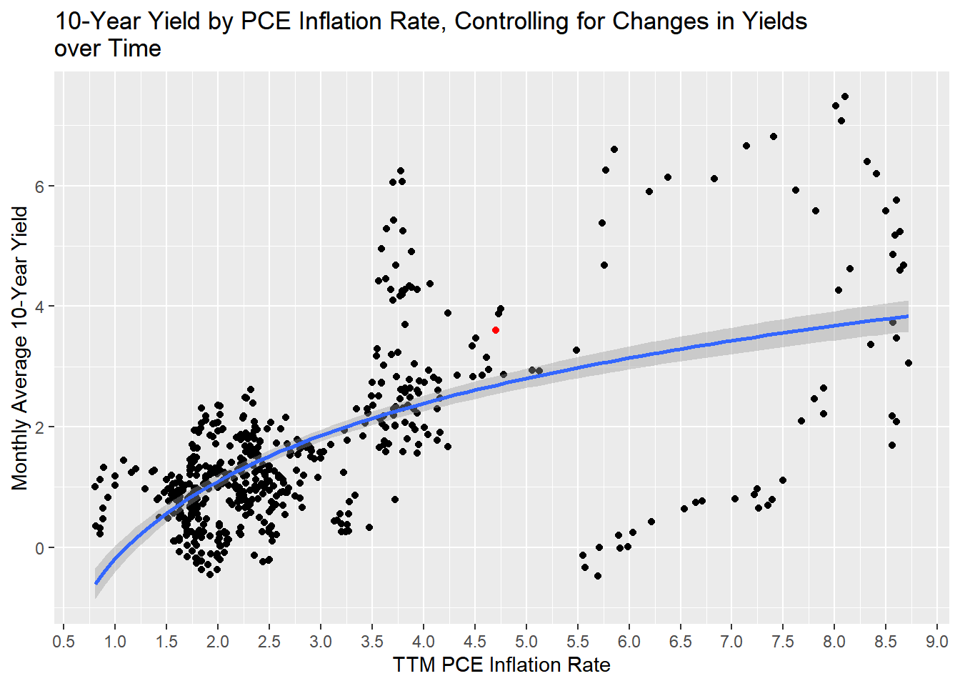
To be sure, the 10-year yield could go much higher. The dispersion of data on our chart is wide. However, this analysis suggests that the 10-year bond may be fairly priced or even slightly underpriced for the current level of inflation, making this a reasonable time to invest in 10-year bonds.
Implications for Stock Market Valuations
The 10-year Treasury yield also has implications for stock market valuations, since it is the “risk-free rate” against which investors measure the attractiveness of stocks’ earnings yields. Can we extend our model, then, to determine if stocks are cheap?
We begin by scraping historical S&P 500 P/E (price-to-earnings) ratios from multpl.com. We join this with our historical PCE inflation rate and 10-year yield data and run a five-fold cross-validation to determine what combination of log or linear regression minimizes error in predicting P/E from inflation rate and 10-year yield.
Double linear: 11.58
Double log: 11.85
Linear PCE, log yield: 11.69
Log PCE, linear yield: 11.67
The winning model is a double linear regression. We retrain this model on the whole dataset and predict P/E. Based on today’s 10-year yield and PCE inflation rate, S&P 500 P/E should be 20.8. This is slightly higher than the actual P/E of 20 (represented by the red dot in the chart below), which suggests the S&P 500 is slightly undervalued.
Furthermore, we can also predict that fair value for the S&P 500 would be even higher if the 10-year yield were to come down from its current 3.6% rate to the 2.7% rate predicted by our yield forecasting model. In that event, we would expect S&P 500 P/E to rise to 21.8 (represented by the green dot in the chart below).

We can thus conclude that the S&P 500, like the US 10-year bond, may be moderately undervalued here.
While these models don't make a strong bull case, they at least suggest buyers won't be grossly overpaying for stocks or bonds at current prices.
Bibliography
Board of Governors of the Federal Reserve System (US). 2022a. “Market Yield on u.s. Treasury Securities at 10-Year Constant Maturity, Quoted on an Investment Basis [Dgs10].” FRED. Federal Reserve Bank of St. Louis. https://fred.stlouisfed.org/series/DGS10.
———. 2022b. “Trimmed Mean PCE Inflation Rate [Pcetrim12m159sfrbdal].” FRED. Federal Reserve Bank of St. Louis. https://fred.stlouisfed.org/series/PCETRIM12M159SFRBDAL.
Boysel S, Vaughan D (2021). fredr: An R Client for the ‘FRED’ API. R package version 2.1.0, https://CRAN.R-project.org/package=fredr.
Garrett Grolemund, Hadley Wickham (2011). Dates and Times Made Easy with lubridate. Journal of Statistical Software, 40(3), 1-25. https://www.jstatsoft.org/v40/i03/.
R Core Team (2022). R: A language and environment for statistical computing. R Foundation for Statistical Computing, Vienna, Austria. https://www.R-project.org/.
“S&P 500 PE Ratio by Month.” multpl. December 31, 2022. https://www.multpl.com/s-p-500-pe-ratio/table/by-month.
Wickham H (2022). rvest: Easily Harvest (Scrape) Web Pages. R package version 1.0.3, https://CRAN.R-project.org/package=rvest.
Wickham H, et al. (2019). “Welcome to the tidyverse.” Journal of Open Source Software, 4(43), 1686. https://doi.org/10.21105/joss.01686.
RMarkdown code (Github)
PDF version (Github)